Post 6: Python

Background
Python is an open source programming language used to write scripts for ArcGIS.  With the current shift in focus towards interoperability, Python usage is becoming increasingly common as it can be used and distributed by third parties.  Because Python works as both a scripting and programming language, it is capable of running everything from simple scripts to complex, advanced programming tasks.  Additionally, Python scripts are run from the source, directly from the script, which makes them more portable and easier to use than other programming languages (Zandbergen, 19).  The versatility and open accessibility of Python ensure it has a bright future and make it a valuable tool for all GIS users to have.  Thus, our class spent some time working with writing Python script.

Goal
The goal of these exercises was to become familiar with the uses of Python and develop a basic level of proficiency with writing script.

Scripts
In addition to completing several tutorials, we wrote multiple standalone scripts to demonstrate our understanding of Python.

Exercise 1. This script converts coordinates for points from a geographic coordinate system to UTM.

Exercise 5/Python Exercise 6. This script prints the name and geometry of all feature classes in a workspace, such as "road is a line."

Exercise 5/Python Exercise 7. First, this script selects all points designated as airports and creates a 15,000 meter buffer around them. Then, the script selects all points designated as seaplane bases and creates a 7,500 meter buffer around them.  Thus, two new feature classes are created.

Source
Zandbergen, Paul. Python Scripting for ArcGIS. 1st. Redlands: Esri Press, 2013. 19. Print.

Post 5: Raster Modeling

Overall Goal
The goal of this portion of the project was to create frac sand mining suitability and environmental/cultural risk models for Tremeapleau County using geoprocessing tools and model builder.  Each model accounts for several important factors, and when joined together, the two models can be used to create a single model for determination of ideal mining locations.


Suitability Model 

Objectives
The objective of the sustainability model was to create layers that account for/rank geology, land cover, distance to the nearest railroad station, slope, and water table depth according to their effect on the suitability of a region for frac sand mining.  The rankings associated with each layer were combined, creating a single, comprehensive suitability index model.  Additionally, any area with land use unsuitable for mining was removed from the ranking.

Data Sources
Data came from a variety of sources, which included past project work, as well as publicly accessible data sets. County/state and bedrock geology data were provided by the professor. Land cover data was downloaded from the NLCD website, rail loading points were generated, and an elevation raster was created in class for exercise 4. Water-table information was downloaded from the Wisconsin Geological Survey.

Methods
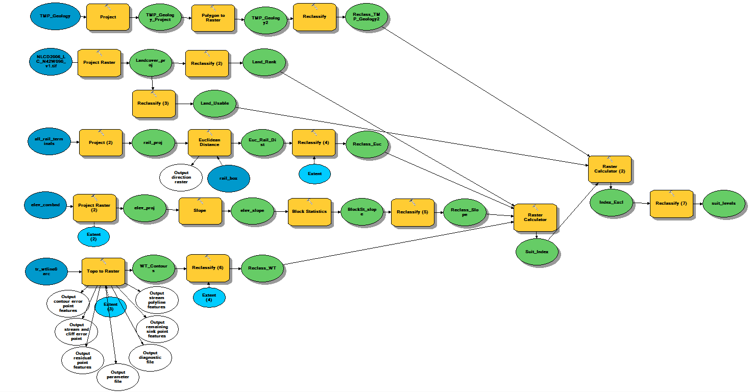
The first step for each layer was ensuring they were in the correct projection (Fig. 6).  I used the county projection system specific to Trempealeau (NAD_1983_HARN_WISCRS_Trempealeau_County_Meters). For the geology layer, I had to convert the initial polygon features to a raster and reclassified the values.  Because the Jordan and Wonewoc are the only formations suitable for frac sand production, they were given a value of 1.  All other formations were given a value of 0, indicating no potential for frac sand mining (Fig. 1).

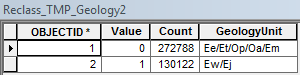
Figure 1.  The Wonewoc and Jordan formations (Ew/Ej) were reclassified as the only geologic units desirable for frac sand mining.

The land cover data required two separate reclassifications (Fig. 2).  One reclassification generated a raster with three separate rankings.  Developed areas and open water were given a value of 1 (low suitability). Forested areas, wetlands, and cultivated/agricultural land were given a value of 2 as they could be mined, but would require some additional effort intially.  Baren, shrubland, and herbacous areas were given a value of 3 (high suitability) because they could be cleared and ready for mining with minimal effort. The second reclassification was used to create a raster that separated out developed and water filled areas, as they are essentially unmineable.

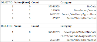
Figure 2.  The top table was used to rank land cover based on suitability for mining. The bottom table was created to allow for the removal of developed and water filled areas from the model.

Euclidean distance was used with the rail terminal data to determine how far each cell in the Trempealeau County raster was from the nearest rail loading point. The raster was then reclassified to create three rankings (Fig. 3).  Because the perceived inconvenience of truck transport is related to the availability of alternative options, I used Jenks' natural breaks and gave cells farthest from rail access a value of 1 and those closest a value of 3.

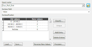
Figure 3.  Reclassification of euclidean distance data (in meters) for rail loading points. 

Elevation data from exercise 4 was run through the slope tool to determine flatter, more convenient mine options.  Block statistics were used with a 3 cell by 3 cell rectangle that calculated the mean to smooth out the data and eliminate any "salt and pepper" effect (Fig. 4). Steep slopes were given a value of 1 (least suitable) and flat areas were given a value of 3 (most suitable).

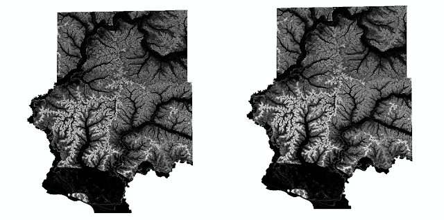
Figure 4.  The original slope raster (left) and the smoother slope raster generated using block statistics (right).

Depth to water level data had to be imported as a coverage.  Topographic data was then converted to a raster based on the elevation of the water table.  Because the frac sand mining process requires significant water supplies, shallow water table elevations were assigned a value of 3 (most suitable) and deep water table elevations were assigned a value of 1 (least suitable) (Fig. 5).

Figure 5.  Water table elevations (old values) were used to classify the suitability of areas for frac sand mining based on the availability of water.

Raster calculator was used to add the values for the land cover, rail distance, slope, and water table depth rankings ("%Reclass_WT%" + "%Reclass_Slope%" + "%Reclass_Euc%" + "%Land_Rank%").  The sum was then multiplied by the geology and usable land rasters to eliminate areas where mining wasn't feasible ("%Suit_Index%" * "%Land_Usable%" * "%Reclass_TMP_Geology2%"). Finally, the values were reclassified using Jenks' natural breaks to determine areas of high, medium, and low suitability (Fig. 13)

Figure 6.  A model for determining frac sand mining suitability based on geology, land cover, rail distance, slope, and water table depth.

Environmental/Cultural Impact Model 

Objectives
The objective of the sustainability model was to create layers that look at the effect on streams, agriculture, residential areas, schools, and parks based on proximity to mining locations.  The values from each layer were divided into three categories 1 (low impact), 2 (med impact), and 3 (high impact).  The rankings for all the layers were combined, creating a single, comprehensive risk model.  Additionally, any area within 640 meters of residential locations (noise/dust shed) was removed from the model.

Data Sources
Data for this portion of the project came from two different sources. Stream and land use data was downloaded from the DNR website. Residential, school, and park locations were provided by ESRI. Populated places (ESRI) was used for residential data. This data is beneficial in that it focuses on main population centers.  However, it does not adequately account for rural homes that tend to be more isolated.

Methods
As in building the suitability model, the first step for each layer was ensuring they were in the correct projection (Fig. 10).  To stay consistent, I again used the county projection system specific to Trempealeau (NAD_1983_HARN_WISCRS_Trempealeau_County_Meters).  For the stream data, I removed the overland flow categories, as overland flow is considered runoff rather than stream flow in the hydrogeologic community. Beyond that, the processing of most layers stayed similar. Euclidean distance was used to generate four rasters showing the distance from each cell to streams, populated/residential areas, schools, and parks. Possible mine locations close to features were assigned values of 3 (high impact) while those further separated were given value of 1 (low impact) using the reclassify tool.

Land cover data was evaluated differently because the concern is for farming potential of potential mine locations rather than proximity (Fig. 7). Croplands or areas that are already being used for agriculture were given a value of 3 (high impact).  Forested and vegetated areas that had the potential to be turned into farm land, which were the majority, were given a value of 2 (med impact).  Developed areas and those with open water were given a value of 1 (low impact) as they are very unlikely to be used for agricultural purposes.

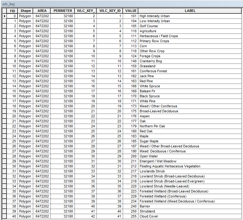
Figure 7.  Land cover data was reclassified based on farming potential (LABEL).

An additional reclassification of proximity to populated areas was run to create a dust/noise shed buffer (Fig. 8). Areas within 640 meters of residential locations were given a value of 0, and areas outside the buffer were given a value of 1.

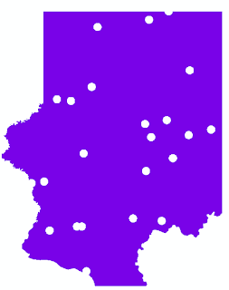
Figure 8.  640 meter buffer areas (white, circular holes) were removed from the model around populated locations. 

The rankings of stream, school, residential, and park proximity, as well as farm potential (prime_farm), were summed using raster calculator to generate a risk index ("%park_reclass%" + "%school_reclass%" + "%populated_reclass%" + "%prime_farm%" + "%stream_reclass%").  These values were then multiplied by the dust/noise shed buffer ("%index_model%" * "%noise_shed%") to eliminate any areas within the unmineable zone. Finally, the raster was reclassified using Jenks' natural breaks to produce three overall impact rankings (high, med, low) (Fig. 15).

As a side project, the viewpath tool was run to determine if any mining locations would be visible from the Arcadia Country Club (Fig. 9).  Clearly, visibility extends miles beyond the actual site.  This likely indicates a frac sand facility in this area would alter the scenery, even from significant distances.

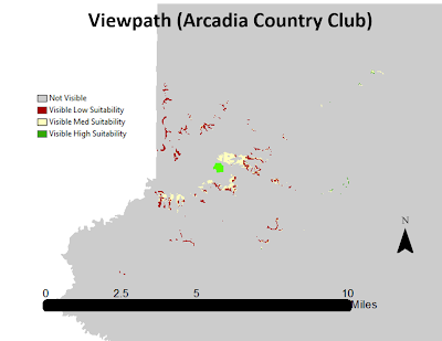
Figure 9.  Visibility clearly extends several miles away from Arcadia Country Club (lime green) in all directions.

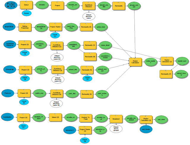
Figure 10.  A model for determining the environmental/cultural risks associated with frac sand mining locations.

Overlay (Combined) Model 

Objectives
The objective of the overlay model was to combine both the suitability and risk models to determine ideal locations for frac sand mining that pose minimal environmental/cultural risk.

Data Sources
Data came from the suitability and risk models, which were based on the various sources described earlier.

Methods
As all data was in the correct projection, no additional projection was necessary (Fig. 11). In order to find areas with high suitability and low risk, the risk model was reclassified so that low risk areas were assigned higher values and high risk areas lower values (flipped from original).  The values of the two models were then multiplied together to determine potential for mining.  The highest potential areas had a value of 9, and the lowest potential areas had a value of 1. The combined values were then reclassified into three categories (high potential, medium potential, low potential) using Jenks' natural breaks (Fig. 16).

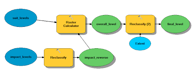
Figure 11.  The final combining of both the suitability and risk model into a single model for determining ideal frac sand mining locations.

Results

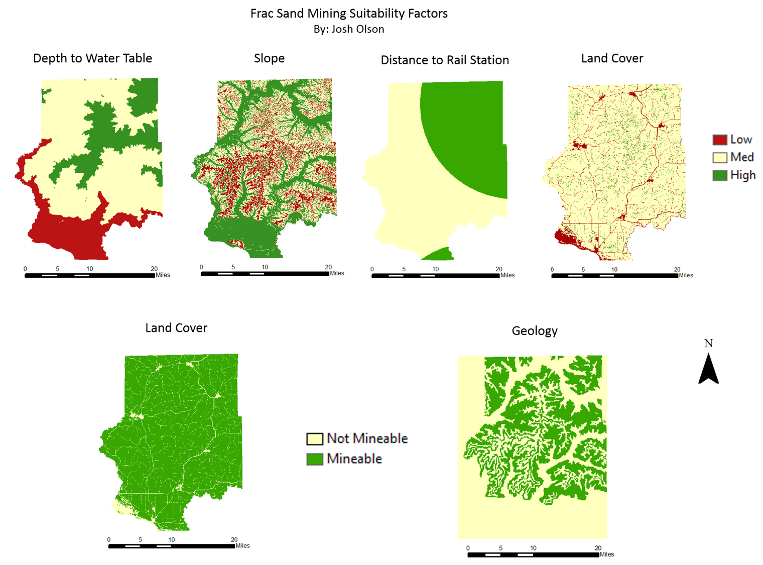
Figure 12. Maps of suitability factors ranked high-low suitability (top) or mineable/not mineable (bottom).

The various factors that account for mine suitability vary greatly in the areas they recommend for mining (Fig. 12). Based on geology and land cover, much of the county is mineable. There appears to be a possible trend of higher suitability in the northeast and lower suitability in the southwest when looking at the water table, rail station, and land cover data.

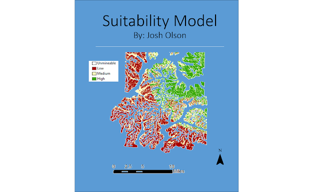
Figure 13. Suitability model created by summing the various suitability factors.

When all of the factors are combined, the trend that was only somewhat visible initially becomes more apparent (Fig. 13).  The northeast corner of the county is clearly the best suited for frac sand mining.  It is interesting how the shape of the distance to rail data was preserved in the northeast, while the small circle fragment in the south is essentially gone. This likely indicates that, not only does distance to rail play a significant role in suitability, but other factors are contributing as well.

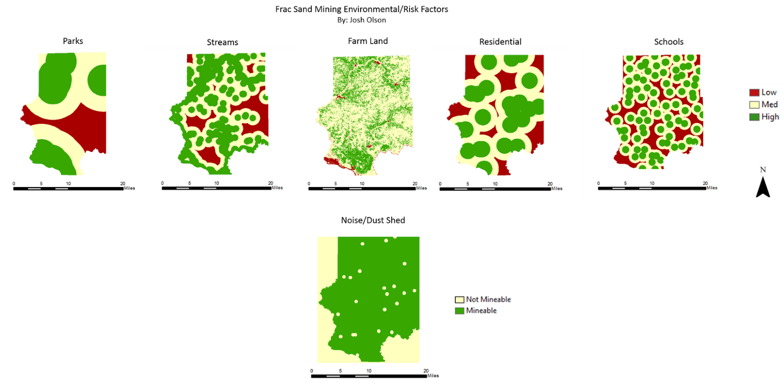
Figure 14.  Maps of risk factors ranked high-low risk (top) and mineable/not mineable (bottom).

Similar to the suitability factors, the risk factors do not immediately indicate a preferred region for mining. Different factors show lower risks in differing areas (Fig. 14).

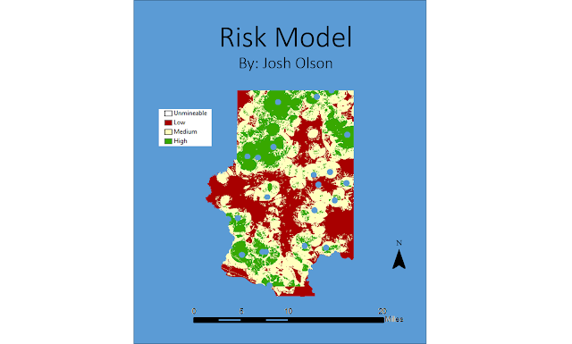
Figure 15. Risk model created by summing the risk factor values.

When all the risk factors are combined, it appears the area of lowest risk is a stretch across the central part of the county (Fig. 15).  This creates potential issues, as it is a somewhat different recommendation than was presented by the suitability data.

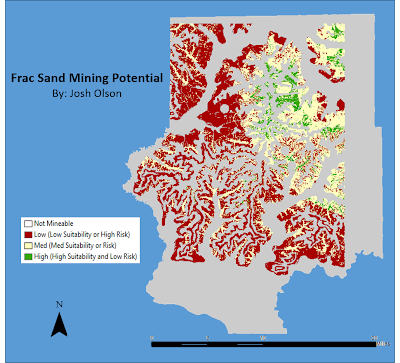
Figure 16. Complete model that accounts for both suitability and risk in determining mining potential.

When both models are combined into one complete model, a better understanding develops.  The high suitability of the northeast corner is clearly shown, and the low risk section across the center of the county is largely masked by less than ideal suitability. The outside perimeter of the county appears to be the most likely region to not be mineable.

Conclusions
This exercise was  valuable because it demonstrated the importance of looking at all the factors in a situation when drawing conclusions.  Though each individual suitability/risk factor presented some bit of information, the big picture was rather unclear when looking at the mass of individual factors.  However, by using geoprocessing tools and raster functionality, the individual factors were combined into useful information.  In this case, the potential of the northeast portion of the county for mining is apparent.  It would be interesting to see how the data would change if an additional rail location was added in the county, as it one of the more alterable factors in the model. Overall, the models demonstrate the potential of GIS to assist in decision making in a multi-million dollar industry.

Sources
WDNR - ftp://dnrftp01.wi.gov/geodata/

Post 4: Routing

Objectives
As discussed in the introductory post for this project, one of the concerns associated with frac sand mining in Wisconsin is increased truck travel for sand transportation purposes. This issue forces residents of typically rural areas around mines to adjust to the increased noise and heavier traffic (WDNR, 2012).  In addition, trucks transporting frac sand create substantial wear on local roads that each county is responsible for maintaining. The goal of this portion of the project was to use network analysis to generate probable routes of truck transportation from frac sand facilities to rail terminal locations and assess the annual road repair cost each county would likely sustain as a result.

To complete this objective, data was collected from a variety of sources.  Professor Hupy compiled the results of the class geocoding exercise into a single feature class to represent all frac sand facilities in Wisconsin (Fig. 1).  Additionally, Professor Hupy provided a feature class with all the rail terminals in Wisconsin as well.  The street network dataset came from ESRI street map USA. State and county boundary data also came from ESRI.  Using all of this information, various network analysis and model builder techniques were utilized to determine transportation routes and probable repair costs.




Figure 1. The compiled geocoded locations of all frac sand facilities in Wisconsin.

Methods
The first part of the routing process was determining which frac sand facilities had direct access to rail terminals.  Facilities that were classified as rail loadouts were queried from the geocoded locations.  The accuracy of this classification was then visually verified using ESRI railroad data (Fig. 2).  Frac sand facilities that were also rail loadouts were then merged with the rail terminal feature and removed from the geocoded mine list to ensure no additional transportation costs were accidently estimated for those sites. Locations that were proposed or in development were assumed to not have rail access.



Figure 2.  An example of a frac sand facility that operated as a rail loading terminal and fell directly on the ESRI railroad feature (lower) and a facility that had to transport by truck to the nearest terminal (upper).

In order to use network analysis, the network analysis extension had to be turned on and the network analysis toolbar added (Fig. 3).  Some time was spent becoming familiar with the network analysis features, such as adding locations, generating routes, and finding the nearest facility with the available data.  This understanding was used to help build a model that would generate probable truck transportation routes.

Figure 3. The network analyst extension had to be turned on and the network analyst toolbar added in order to use the desired network analyst tools.

Using model builder, a complete model was constructed that carried out the entire analysis from route generation and length estimation to projected annual costs for each county (Fig. 4).

Figure 4. A model was constructed to single-handedly generate truck transportation routes from each mine to the nearest rail terminal, calculate the total route length in each county, and estimate the annual repair cost associated with the truck travel.
(W:\geog\CHupy\geog337_f13\OLSONJC\Ex_7\Ex_7.gdb\Toolbox\Ex_7)

The "Make Closest Facility Layer" tool was first added to the model (top left of Figure 4) using the streets network data set for routing.  The geocoded mine locations were added as the incidents layer, and the rail terminal locations were added as the facilities layer.  This allowed the closest facility tool to be solved and generate routes from each mine to the nearest rail terminal, using the streets network dataset. Routes were then selected out and a copy of the routes feature class was added to the geodatabase (moving down right side of Figure 4).  Because the routes and county feature classes were in geographic coordinate systems, they had to be projected to ensure accuracy in route distance estimation. The project tool was used to project the routes and county feature classes in the UTM Zone 15N coordinate system.  Even though some of the mines are technically in UTM Zone 16N, UTM Zone 15N was used to stay consistent with the projection of the geocoded mines. Because the goal was to estimate repair costs for each county, the intersect tool was used to break routes at county boundaries and join the two data sets together.  However, this generated several route fragments in each county, which needed to be grouped for estimation of total route distance. To do this, the frequency tool was used, grouping the route fragments by county name and summing the shape length for all routes in the same county.  Because we were using a UTM projection, this step provided total route distance in meters.  Another field was added (Truck_Mile_Year) to convert the total route distance to miles and factor in the number of total truck trips.  Professor Hupy designated an estimate of 50 truck trips each year.  As the trucks must drive to the rail terminal and back, total route distance would be covered 100 times.  Thus, the calculate field tool was used with the equation:
"Truck_Mile_Year = Shape Length*0.000621371*100". 
This equation both compensates for conversion for meters to miles and total truck trips each year. The final calcution was the estimate of annual cost for each county.  Professor Hupy designated a cost of 2.2 cents per mile ($0.022). As the total travel distance was already converted to miles, this step simply involved creating another field in the table (Truck_Cost_Year) and using the calculate field tool to run the equation: 
"Truck_Cost_Year = Truck_Mile_Year*0.022".
This populated the "Truck_Cost_Year" field with estimated annual road repair costs for each county (Fig.5 ).

Results

Figure 5. Analysis results were compiled in a single table that gave annual truck miles and cost per year for each county.

The results indicate that only 26 of the 72 counties in Wisconsin will experience increased truck traffic due to frac sand transportation (Fig. 6). Of the 26 counties, Outagamie is the least affected, paying just over $1 annually to compensate for 47 miles of truck travel. Interestingly, Trempealeau county, the focus of the project, is the most affected with almost 40,000 truck miles annually and $878 in road repair costs (Fig. 7). 

Figure 6.  Trucking routes covered 26 counties in Wisconsin, with an obvious focus on the western edge of the state.



Figure 7. Trempealeau county has the most truck traffic of any county in the state. Rail terminals appear to be uncommon in this area, which likely results in the extensive transportation of frac sand by truck.

Though our data has some error associated with the original geocoding process and unaccounted for proposed rail terminals, the results are as one would expect: the western edge of the state is the most affected by truck transportation.  This is primarly due to the high density of mines in this region.  Road repair costs seem to be fairly well spread among the counties according to the number of mines.  While Trempealeau county would be expected to have a relatively high repair cost based on the number of mines, the infrequency of rail terminals in the area appears to be increasing truck travel.  This also seems to be the case for the cluster of mines southeast of Trempealeau.  Both areas would benefit from the addition of a centrally located rail terminal to reduce transportation costs for many of the mines.  Based on the small amount that each county has to contribute currently, it is unlikely that any county would make such an investment.  Thus, the mining or railroad companies would likely have to provide the resources. 

Conclusions
Though cost per truck mile was based on an unverified value and requires additional research, the network analysis and model builder tools indicate that the economic costs of truck transportation is rather insignificant.  Considering the millions of dollars spent in the frac sand industry each year, each county could charge a small tax that would be essentially negligible to mining companies.  Though this does not address potential inconvenience to citizens, it would allow counties to maintain roads at no out-of-pocket cost.  Additionally, the routes revealed some inefficencies in current transportation methods.  There are relatively few rail terminals in the western part of the state, forcing many mines to use truck transportation for significant distances. The addition of central rail terminals in these areas should be considered for economic and convenience purposes. Because frac sand mining is so rapidly evolving across the state, which alters rail access as well, information must be constantly updated to properly evaluate ideal transportation routes and future rail terminal locations.

Sources
WDNR. (2012, JANUARY). Silica sand mining in wisconsin. Retrieved from

            http://dnr.wi.gov/topic/Mines/documents/SilicaSandMiningFinal.pdf

Post 2: Data Gathering

Goals and Objectives
The goal of this exercise was to learn how to download data from a variety of publicly accessible websites and manipulate the data into a form that was functional for our purposes. To do this, we needed to import the downloaded data into ArcGIS and join where appropriate. Finally, all data had to be compiled into a single geodatabase with the same projection.  The processed data will serve as the base data for our ongoing Trempealeau County frac sand project.

General Methods
Four different online sources were used to collect railroad, land cover, elevation, cropland, and soil data. These included the US National Atlas, USGS National Map Viewer, USDA Geospatial Data Gateway, and USDA NRSC Web Soil Survey (SSURGO) (Fig.1).

Figure 1. The data was downloaded from a variety of online sources.

To receive the data, various requests and form submissions were required at each site, which generally resulted in the download of a zip file.  The files had to be unzipped and desired files located.  This was not always straightforward. For example, the elevation data provided by the USGS National Map Viewer was delivered in multiple files due to the size of the data.  As we wanted a single elevation raster, we had to join the two DEMs together using the mosaic tool.  This step required we use the appropriate bit depth, so as not to lose any data in the process. Also, the SSURGO soil shapefile we wanted had to be imported into a feature class in our geodatabase. We then joined the soil information from the "component" table to the feature class based on a relationship class we created. Additionally, we joined drainage index and productivity index tables to the SSURGO data, using DI index as the symbology for the feature.

The data quality varied for each source and data set.  To ensure proper use of the data later in our project, data quality information was compiled from the metadata of each data set (Fig. 2)

Figure 2.  The data sets vary in quality, which will be important to be aware of in later aspects of the project.

Results
With all desired data collected, the final step was to project all the features in the same coordinate system. As our study focuses on Trempealeau County, I used "NAD 1983 UTM Zone 15N" as my projected coordinate system. To do this, I used the "project raster" tool for the land cover, elevation, and cropland features and the "project" tool for the railroad and soils data (Fig. 3). All the data sets appear to have been processed correctly.  They should work well as the base data for later project analysis.

Figure 3.  Layers are shown individually, as well as together (upper left).  

Sources
Concepts and Techniques in Geographic Information Systems
CP Lo, AKW Yeung - 2003 - Pearson Prentice Hall

Post 3: Geocoding

Goals and Objectives
For this portion of the project, our goal was to download frac sand facility location data from a county website (www.tremplocounty.com), as well as a statewide website (WisconsinWatch.org), which was in the form of an Excel file.  We then had to normalize the data and geocode the assigned locations. After all the results were geocoded, matching locations that were geocoded by different users were compared to demonstrate error that can occur in the geocoding process.

Methods
Geocoding involves assigning coordinates or an address for a specific data point.  We attempted to geocode the locations of all known frac sand facilities (proposed and functioning) in Wisconsin based off data provided by WisconsinWatch.org.  The data were in the form of an Excel table with various types of addresses given.  In order to allow the geocoder to run the given addresses, we first had to normalize the table.  We then ran the program to see which locations could be matched and which locations would require further investigation and manual placement or address format changes to be located properly.

For addresses that had a full street address and could be matched, we simply selected the appropriate location and an address was automatically assigned to the point. However, this only worked on 4 of the 14 points, so alternative methods were required. For addresses that were given in the form of a generic or PLSS description, I used Google Earth and a PLSS coordinate converter to attempt to determine a street address, which could be matched in the Geocoder.  This worked for three of my data points. For the remaining seven locations, I used the "pick the address from the map" feature in the Geocoder to manually place the point.  I then manually updated the address information in the table as well.

Results
The initial Excel file downloaded from WisconsinWatch.org was very cluttered with confusing and unnecessary information (Fig. 1).

Figure 1.  The original table had many inconsistencies and additional information that required normalization.

In order to make the data usable, we normalized the table.  This entailed making sure all attributes were functionally dependent on the unique primary key (UNIQUE ID) and minimizing the storage of data to ensure data integrity.  To do this, we separated the address into separate fields of facility address, city, zip code, and state categories (Fig.2 ). We then eliminated all fields except for "UNIQUE ID," "Facility Type," "Facility Address," "City," "Community (City)," "Zip Code," and "State." This removed the excess fields and and made all categories directly dependent on the "UNIQUE ID" field. Finally, we made sure that all facility addresses were in the same format.

Figure 2.  After normalizing the data, information is much more clear and usable.

After normalizing the data and filling in any informational gaps using Google Earth and the mining company websites, the frac sand facility locations were all geocoded properly using both geocoder matching and manual placement (Fig. 3).

Figure 3.  After normalization of the data and filling of informational gaps, all 14 frac sand facilities were properly geocoded.

Geocoding results varied significantly depending on the user.  Errors occurred at all stages of the geocoding process and were both inherent and operational in nature.  For example, our original source data were inherently flawed as the setup for providing the information was insufficient for collecting all the necessary address information.  In addition, there was operational error during our data compilation stage.  There were clearly errors made during attribute data input, as some of the addresses placed the facilities in communities that were incorrect or only near the correct city.  Also, each user digitized the locations differently.  This likely resulted from different user interpretation of Google Earth images regarding frac sand facility locations. The differences varied from a few a hundred to over twenty thousand meters (Fig. 4).

Figure 4.  Insufficient source data and differences in digitization resulted in significant variation in users' geocoding                         results. These two points, which are supposed to be the same location, were generated by two different users and are more than 2700 meters apart.

To assess how significantly these sources of error affected the final data, we used the point distance tool. This provided the distance to the point nearest my designated location for a given facility (Fig. 5).  Of the five facility locations I compared, only one matched exactly.  However, this point was matched directly by the Geocoder. The other four points that I compared, which were placed manually, varied from a separation of ~400 meters to ~25,000 meters.  Unfortunately, this data processing tool has inherent error, as it does not find points based on matching primary keys, but uses proximity alone.

Figure 5.  The point distance tool was used to assess the impact of inherent and operational error on the final data by                       measuring the distance from a specified facility location (INPUT_FID) to the nearest point generated by another user (NEAR_FID).

Conclusion

Though the original data table was quite unclear and lacking in information, we were able to generate adequate geocoding results by using normalization and some help from Google Earth and additional research. However, the final product was imperfect, containing significant inherent and operational error. This problem is not uncommon.  In order to verify complete accuracy of location placement, each point should be compared to reference data with a higher degree of accuracy.  If no such data is available for the frac sand facility locations, coordinates should be manually collected at each site and then compared to reference data points in the area, ensuring the accuracy of each location.

Post 1: Overview

Frac Sand and Hydraulic Fracturing

Discussion of the material known as “frac sand” has become increasingly common in recent years, especially in Wisconsin. This leads to the question, "What exactly is frac sand, and why is it so significant?" Frac sand is used for oil and natural gas extraction in a process known as hydraulic fracturing. Hydraulic fracturing involves pumping a slurry of water, chemicals, and sand under high pressure, deep into oil and natural gas wells in order to expand naturally-occurring or explosive-induced fractures within shale formations. After the pressure is released, the frac sand grains remain behind, acting as pillars that keep the fractures propped open and permit oil and gas to flow more freely from the formation. This technology has been known for the last 75 years.  However, its potential has only recently been realized with advancements in horizontal drilling.  Combining the two techniques (Fig. 1) has drastically increased oil and gas extraction abilities and allowed formations that were previously too expensive to drill to become profitable (WDNR, 2012).



Figure 1.  An illustration of combining hydraulic fracturing and horizontal drilling to enlarge fractures in shale formations to more easily remove oil and natural gas (WDNR, 2012).

The hydraulic fracturing process requires a very specific type of sand.  Effective frac sand must be almost pure quartz, so it is strong enough to hold the weight of the overlying material. Additionally, the sand grains must be well rounded, uniform, and sufficiently coarse to create openings in the fractures that are large enough for the oil and natural gas to flow through (WDNR, 2013). Sand meeting these specifications is only formed in specific geologic environments. Wisconsin has multiple sandstone formations that meet the requirements for frac sand and are close enough to the surface to be mined (WDNR, 2012).

Frac Sand Mining in Wisconsin

Mining of frac sand in Wisconsin has primarily been focused in the west-central part of the state (Fig. 2).  In this region, the Jordan, Wonewoc, Mt. Simon, and St. Peter formations all contain sand with the desired traits and are accessible from hilltops and hillsides (WDNR, 2012). Because of the recent surge in demand for frac sand, both nationally and internationally, and Wisconsin’s abundant supply, frac sand mining has become a major contributor to the state’s economy.  There are over 100 frac sand operations active in Wisconsin. These mines and processing facilities have resulted in the creation of over 2,000 jobs, which generate millions of dollars in income and tax revenue. Communities across the state have benefitted from the money brought in by the frac sand industry. Future prospects show no signs of slowing down, but not all Wisconsin residents are excited about this reality (Nichols, 2013).



Figure 2.  Locations of sandstone formations, frac sand mines, and frac sand processing plants across Wisconsin (WDNR, 2013).

Concerns with Frac Sand Mining

Frac sand mining in Wisconsin comes with certain disadvantages and risks.  Many citizens are concerned about mining away the hills that serve as aesthetic icons of the region and how that could affect erosional patterns. Additionally, explosives are used to remove sand for processing, where it is crushed and sorted.  These processes generate significant dust, which can lead to respiratory issues, particularly if the dust is silica-rich.  The most common concern is silicosis, an irreparable respiratory disease caused by the inhalation of fine silica particles. In an effort to control dust, most frac sand operations use a notable amount of water to spray down the plant.  Add this to water already being used to wash the mined material, and the water toll on a region can be considerable, even if the plant is using a closed-loop system. Beyond this, chemicals are used throughout the mining process as flocculants.  If mishandled, these chemicals have the potential to contaminate local groundwater resources. Furthermore, operating such large facilities can generate substantial air emissions. If not properly filtered, this can reduce local air quality, as well as release greenhouse gases. In addition to health and safety issues, frac sand facilities can be inconvenient for facility neighbors in other ways (WDNR, 2012).

Removal, processing, and transportation of frac sand creates ongoing inconveniences typically not experienced in many rural communities.  Facility, equipment, and train operations often generate ongoing noise and light that can last throughout the night.  Also, frac sand is commonly transported in large dump trucks on roads that previously saw very little traffic (WDNR, 2012).  This is a change locals have to adjust to and has the potential to generate a higher number of serious accidents in the area.  Because of these issues, along with the other health concerns discussed, many locals fear the value of their homes will decrease drastically if a frac sand plant is opened nearby (Nichols, 2013).

In-Class Risk Assessment

Clearly, frac sand mining is an important issue in Wisconsin.  It has high-risk potential, but high-reward potential as well.  Because of this, it is important to build a thorough suitability/risk model for frac sand mining in Western Wisconsin.  This will be the focus of our class project, with a particular emphasis on Trempealeau County. To complete this task, we will download data from a variety of sources, such as the National Atlas, the USGS, and the USDA. Using these resources and a variety of data analysis methods, we will hopefully be able to generate a useful, accurate model.

Sources

Nichols, M. (2013, April). Mining success. Wisconsin Interest, 22(1), Retrieved from
            http://www.wpri.org/WIInterest/Vol22No1/Nichols22.1.html

WDNR. (2012, JANUARY). Silica sand mining in wisconsin. Retrieved from
            http://dnr.wi.gov/topic/Mines/documents/SilicaSandMiningFinal.pdf 

WDNR. (2013). Frac sand in wisconsin: Fact sheet 05. Retrieved from  

            http://wisconsingeologicalsurvey.org/pdfs/frac-sand-factsheet.pdf