Post 4: Routing

Objectives
As discussed in the introductory post for this project, one of the concerns associated with frac sand mining in Wisconsin is increased truck travel for sand transportation purposes. This issue forces residents of typically rural areas around mines to adjust to the increased noise and heavier traffic (WDNR, 2012).  In addition, trucks transporting frac sand create substantial wear on local roads that each county is responsible for maintaining. The goal of this portion of the project was to use network analysis to generate probable routes of truck transportation from frac sand facilities to rail terminal locations and assess the annual road repair cost each county would likely sustain as a result.

To complete this objective, data was collected from a variety of sources.  Professor Hupy compiled the results of the class geocoding exercise into a single feature class to represent all frac sand facilities in Wisconsin (Fig. 1).  Additionally, Professor Hupy provided a feature class with all the rail terminals in Wisconsin as well.  The street network dataset came from ESRI street map USA. State and county boundary data also came from ESRI.  Using all of this information, various network analysis and model builder techniques were utilized to determine transportation routes and probable repair costs.




Figure 1. The compiled geocoded locations of all frac sand facilities in Wisconsin.

Methods
The first part of the routing process was determining which frac sand facilities had direct access to rail terminals.  Facilities that were classified as rail loadouts were queried from the geocoded locations.  The accuracy of this classification was then visually verified using ESRI railroad data (Fig. 2).  Frac sand facilities that were also rail loadouts were then merged with the rail terminal feature and removed from the geocoded mine list to ensure no additional transportation costs were accidently estimated for those sites. Locations that were proposed or in development were assumed to not have rail access.



Figure 2.  An example of a frac sand facility that operated as a rail loading terminal and fell directly on the ESRI railroad feature (lower) and a facility that had to transport by truck to the nearest terminal (upper).

In order to use network analysis, the network analysis extension had to be turned on and the network analysis toolbar added (Fig. 3).  Some time was spent becoming familiar with the network analysis features, such as adding locations, generating routes, and finding the nearest facility with the available data.  This understanding was used to help build a model that would generate probable truck transportation routes.

Figure 3. The network analyst extension had to be turned on and the network analyst toolbar added in order to use the desired network analyst tools.

Using model builder, a complete model was constructed that carried out the entire analysis from route generation and length estimation to projected annual costs for each county (Fig. 4).

Figure 4. A model was constructed to single-handedly generate truck transportation routes from each mine to the nearest rail terminal, calculate the total route length in each county, and estimate the annual repair cost associated with the truck travel.
(W:\geog\CHupy\geog337_f13\OLSONJC\Ex_7\Ex_7.gdb\Toolbox\Ex_7)

The "Make Closest Facility Layer" tool was first added to the model (top left of Figure 4) using the streets network data set for routing.  The geocoded mine locations were added as the incidents layer, and the rail terminal locations were added as the facilities layer.  This allowed the closest facility tool to be solved and generate routes from each mine to the nearest rail terminal, using the streets network dataset. Routes were then selected out and a copy of the routes feature class was added to the geodatabase (moving down right side of Figure 4).  Because the routes and county feature classes were in geographic coordinate systems, they had to be projected to ensure accuracy in route distance estimation. The project tool was used to project the routes and county feature classes in the UTM Zone 15N coordinate system.  Even though some of the mines are technically in UTM Zone 16N, UTM Zone 15N was used to stay consistent with the projection of the geocoded mines. Because the goal was to estimate repair costs for each county, the intersect tool was used to break routes at county boundaries and join the two data sets together.  However, this generated several route fragments in each county, which needed to be grouped for estimation of total route distance. To do this, the frequency tool was used, grouping the route fragments by county name and summing the shape length for all routes in the same county.  Because we were using a UTM projection, this step provided total route distance in meters.  Another field was added (Truck_Mile_Year) to convert the total route distance to miles and factor in the number of total truck trips.  Professor Hupy designated an estimate of 50 truck trips each year.  As the trucks must drive to the rail terminal and back, total route distance would be covered 100 times.  Thus, the calculate field tool was used with the equation:
"Truck_Mile_Year = Shape Length*0.000621371*100". 
This equation both compensates for conversion for meters to miles and total truck trips each year. The final calcution was the estimate of annual cost for each county.  Professor Hupy designated a cost of 2.2 cents per mile ($0.022). As the total travel distance was already converted to miles, this step simply involved creating another field in the table (Truck_Cost_Year) and using the calculate field tool to run the equation: 
"Truck_Cost_Year = Truck_Mile_Year*0.022".
This populated the "Truck_Cost_Year" field with estimated annual road repair costs for each county (Fig.5 ).

Results

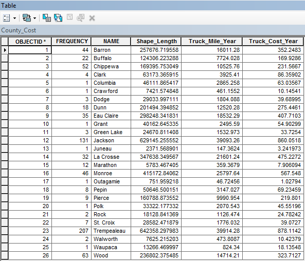Figure 5. Analysis results were compiled in a single table that gave annual truck miles and cost per year for each county.

The results indicate that only 26 of the 72 counties in Wisconsin will experience increased truck traffic due to frac sand transportation (Fig. 6). Of the 26 counties, Outagamie is the least affected, paying just over $1 annually to compensate for 47 miles of truck travel. Interestingly, Trempealeau county, the focus of the project, is the most affected with almost 40,000 truck miles annually and $878 in road repair costs (Fig. 7). 

Figure 6.  Trucking routes covered 26 counties in Wisconsin, with an obvious focus on the western edge of the state.



Figure 7. Trempealeau county has the most truck traffic of any county in the state. Rail terminals appear to be uncommon in this area, which likely results in the extensive transportation of frac sand by truck.

Though our data has some error associated with the original geocoding process and unaccounted for proposed rail terminals, the results are as one would expect: the western edge of the state is the most affected by truck transportation.  This is primarly due to the high density of mines in this region.  Road repair costs seem to be fairly well spread among the counties according to the number of mines.  While Trempealeau county would be expected to have a relatively high repair cost based on the number of mines, the infrequency of rail terminals in the area appears to be increasing truck travel.  This also seems to be the case for the cluster of mines southeast of Trempealeau.  Both areas would benefit from the addition of a centrally located rail terminal to reduce transportation costs for many of the mines.  Based on the small amount that each county has to contribute currently, it is unlikely that any county would make such an investment.  Thus, the mining or railroad companies would likely have to provide the resources. 

Conclusions
Though cost per truck mile was based on an unverified value and requires additional research, the network analysis and model builder tools indicate that the economic costs of truck transportation is rather insignificant.  Considering the millions of dollars spent in the frac sand industry each year, each county could charge a small tax that would be essentially negligible to mining companies.  Though this does not address potential inconvenience to citizens, it would allow counties to maintain roads at no out-of-pocket cost.  Additionally, the routes revealed some inefficencies in current transportation methods.  There are relatively few rail terminals in the western part of the state, forcing many mines to use truck transportation for significant distances. The addition of central rail terminals in these areas should be considered for economic and convenience purposes. Because frac sand mining is so rapidly evolving across the state, which alters rail access as well, information must be constantly updated to properly evaluate ideal transportation routes and future rail terminal locations.

Sources
WDNR. (2012, JANUARY). Silica sand mining in wisconsin. Retrieved from

            http://dnr.wi.gov/topic/Mines/documents/SilicaSandMiningFinal.pdf